Non-Linear Regression Modeling with Bootstrapping: mtcars
Background & Info
This data comes from the R dataset mtcars and is an expansion on the
example given here.
There is not much data in this set, so we can bootstrap the sample to try to get a more robust picture. Bootstrapping is the process of taking random samples of a dataset in order to have multiple sets to model. With enough samples, this should reasonably give us an upper and lower bound that is more reliable that what would be generated from the residuals of the original dataset.
Let’s strap those boots!
library(tidymodels)

print(mtcars)
##                      mpg cyl  disp  hp drat    wt  qsec vs am gear carb
## Mazda RX4           21.0   6 160.0 110 3.90 2.620 16.46  0  1    4    4
## Mazda RX4 Wag       21.0   6 160.0 110 3.90 2.875 17.02  0  1    4    4
## Datsun 710          22.8   4 108.0  93 3.85 2.320 18.61  1  1    4    1
## Hornet 4 Drive      21.4   6 258.0 110 3.08 3.215 19.44  1  0    3    1
## Hornet Sportabout   18.7   8 360.0 175 3.15 3.440 17.02  0  0    3    2
## Valiant             18.1   6 225.0 105 2.76 3.460 20.22  1  0    3    1
## Duster 360          14.3   8 360.0 245 3.21 3.570 15.84  0  0    3    4
## Merc 240D           24.4   4 146.7  62 3.69 3.190 20.00  1  0    4    2
## Merc 230            22.8   4 140.8  95 3.92 3.150 22.90  1  0    4    2
## Merc 280            19.2   6 167.6 123 3.92 3.440 18.30  1  0    4    4
## Merc 280C           17.8   6 167.6 123 3.92 3.440 18.90  1  0    4    4
## Merc 450SE          16.4   8 275.8 180 3.07 4.070 17.40  0  0    3    3
## Merc 450SL          17.3   8 275.8 180 3.07 3.730 17.60  0  0    3    3
## Merc 450SLC         15.2   8 275.8 180 3.07 3.780 18.00  0  0    3    3
## Cadillac Fleetwood  10.4   8 472.0 205 2.93 5.250 17.98  0  0    3    4
## Lincoln Continental 10.4   8 460.0 215 3.00 5.424 17.82  0  0    3    4
## Chrysler Imperial   14.7   8 440.0 230 3.23 5.345 17.42  0  0    3    4
## Fiat 128            32.4   4  78.7  66 4.08 2.200 19.47  1  1    4    1
## Honda Civic         30.4   4  75.7  52 4.93 1.615 18.52  1  1    4    2
## Toyota Corolla      33.9   4  71.1  65 4.22 1.835 19.90  1  1    4    1
## Toyota Corona       21.5   4 120.1  97 3.70 2.465 20.01  1  0    3    1
## Dodge Challenger    15.5   8 318.0 150 2.76 3.520 16.87  0  0    3    2
## AMC Javelin         15.2   8 304.0 150 3.15 3.435 17.30  0  0    3    2
## Camaro Z28          13.3   8 350.0 245 3.73 3.840 15.41  0  0    3    4
## Pontiac Firebird    19.2   8 400.0 175 3.08 3.845 17.05  0  0    3    2
## Fiat X1-9           27.3   4  79.0  66 4.08 1.935 18.90  1  1    4    1
## Porsche 914-2       26.0   4 120.3  91 4.43 2.140 16.70  0  1    5    2
## Lotus Europa        30.4   4  95.1 113 3.77 1.513 16.90  1  1    5    2
## Ford Pantera L      15.8   8 351.0 264 4.22 3.170 14.50  0  1    5    4
## Ferrari Dino        19.7   6 145.0 175 3.62 2.770 15.50  0  1    5    6
## Maserati Bora       15.0   8 301.0 335 3.54 3.570 14.60  0  1    5    8
## Volvo 142E          21.4   4 121.0 109 4.11 2.780 18.60  1  1    4    2
ggplot(mtcars, aes(wt,mpg)) +
  geom_point()
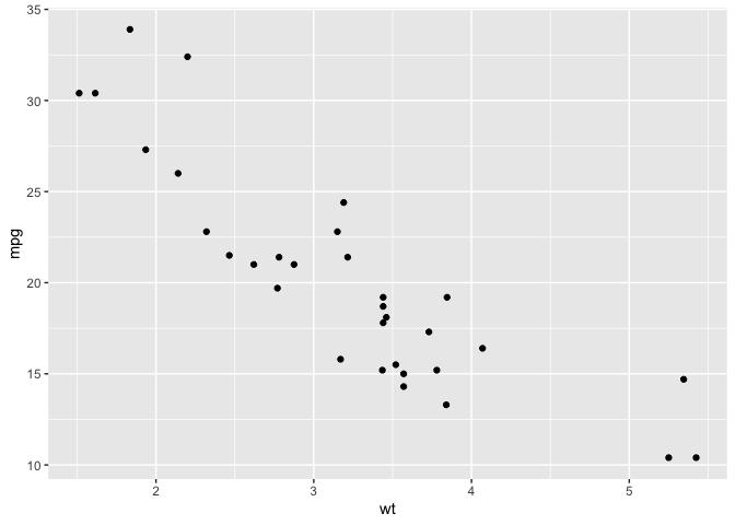
We can see that this data may not have a linear relationship. It seems to follow an \(f(x) = \frac{k}{x} + b\) pattern. The base R function for Nonlinear Least Squares can take this relationship between our response and explanatory variable and give us estimates for k and b.
nls_mdl <- nls(mpg ~ k / wt + b, data = mtcars, start = list(k = 1, b = 0))

ggplot(mtcars,aes(wt,mpg)) +
  geom_point() +
  geom_line(aes(y = predict(nls_mdl)))
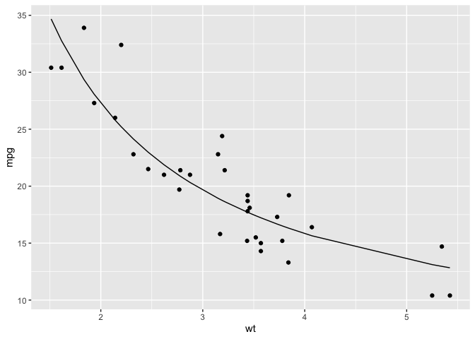
This does seem like a good fit, but again we may be relying too heavily on a data set that does not have many data points. So, by bootstrapping we can simulate a large number of similar samples which, by the Law of Large Numbers, should give us reasonable upper and lower bounds that more closely reflects the population.
Bootstrapping in tidymodels
boots <- bootstraps(mtcars, times = 2000, apparent = TRUE)
boots
## # Bootstrap sampling with apparent sample
## # A tibble: 2,001 x 2
##    splits          id
##    <list>          <chr>
##  1 <split [32/12]> Bootstrap0001
##  2 <split [32/11]> Bootstrap0002
##  3 <split [32/11]> Bootstrap0003
##  4 <split [32/12]> Bootstrap0004
##  5 <split [32/7]>  Bootstrap0005
##  6 <split [32/12]> Bootstrap0006
##  7 <split [32/11]> Bootstrap0007
##  8 <split [32/13]> Bootstrap0008
##  9 <split [32/13]> Bootstrap0009
## 10 <split [32/8]>  Bootstrap0010
## # … with 1,991 more rows
Notice we have a table with a list-column and an id field for each row.
The splits column contains the bootstrapped sample and it is this data
we would like to model for each and every row. Fortunately, and not
coincidentally, the tidymodels family is here to work with this type
of data.
In order to access the data in splits, we use the analysis()
function as follows:
(boots %>%
  slice(1) %>%
  pull(splits))[[1]] %>%
  analysis()
##                        mpg cyl  disp  hp drat    wt  qsec vs am gear carb
## Mazda RX4 Wag         21.0   6 160.0 110 3.90 2.875 17.02  0  1    4    4
## Toyota Corolla        33.9   4  71.1  65 4.22 1.835 19.90  1  1    4    1
## Duster 360            14.3   8 360.0 245 3.21 3.570 15.84  0  0    3    4
## Cadillac Fleetwood    10.4   8 472.0 205 2.93 5.250 17.98  0  0    3    4
## Merc 450SL            17.3   8 275.8 180 3.07 3.730 17.60  0  0    3    3
## Fiat X1-9             27.3   4  79.0  66 4.08 1.935 18.90  1  1    4    1
## Pontiac Firebird      19.2   8 400.0 175 3.08 3.845 17.05  0  0    3    2
## Merc 240D             24.4   4 146.7  62 3.69 3.190 20.00  1  0    4    2
## Lotus Europa          30.4   4  95.1 113 3.77 1.513 16.90  1  1    5    2
## Lincoln Continental   10.4   8 460.0 215 3.00 5.424 17.82  0  0    3    4
## Dodge Challenger      15.5   8 318.0 150 2.76 3.520 16.87  0  0    3    2
## Cadillac Fleetwood.1  10.4   8 472.0 205 2.93 5.250 17.98  0  0    3    4
## Mazda RX4             21.0   6 160.0 110 3.90 2.620 16.46  0  1    4    4
## Pontiac Firebird.1    19.2   8 400.0 175 3.08 3.845 17.05  0  0    3    2
## Ferrari Dino          19.7   6 145.0 175 3.62 2.770 15.50  0  1    5    6
## Mazda RX4 Wag.1       21.0   6 160.0 110 3.90 2.875 17.02  0  1    4    4
## Porsche 914-2         26.0   4 120.3  91 4.43 2.140 16.70  0  1    5    2
## Lincoln Continental.1 10.4   8 460.0 215 3.00 5.424 17.82  0  0    3    4
## Toyota Corolla.1      33.9   4  71.1  65 4.22 1.835 19.90  1  1    4    1
## Porsche 914-2.1       26.0   4 120.3  91 4.43 2.140 16.70  0  1    5    2
## Camaro Z28            13.3   8 350.0 245 3.73 3.840 15.41  0  0    3    4
## Ferrari Dino.1        19.7   6 145.0 175 3.62 2.770 15.50  0  1    5    6
## Porsche 914-2.2       26.0   4 120.3  91 4.43 2.140 16.70  0  1    5    2
## Cadillac Fleetwood.2  10.4   8 472.0 205 2.93 5.250 17.98  0  0    3    4
## Ford Pantera L        15.8   8 351.0 264 4.22 3.170 14.50  0  1    5    4
## Dodge Challenger.1    15.5   8 318.0 150 2.76 3.520 16.87  0  0    3    2
## Lotus Europa.1        30.4   4  95.1 113 3.77 1.513 16.90  1  1    5    2
## Honda Civic           30.4   4  75.7  52 4.93 1.615 18.52  1  1    4    2
## Valiant               18.1   6 225.0 105 2.76 3.460 20.22  1  0    3    1
## Merc 240D.1           24.4   4 146.7  62 3.69 3.190 20.00  1  0    4    2
## Datsun 710            22.8   4 108.0  93 3.85 2.320 18.61  1  1    4    1
## Merc 450SE            16.4   8 275.8 180 3.07 4.070 17.40  0  0    3    3
How would this work in the context of tidymodels though? First, we
need to write a function which will properly extract the data from our
bootstrap set, which technically is an rset object.
bootstrapNls <- function(dat){
  nls(mpg ~ k / wt + b, analysis(dat), start = list(k = 1, b = 0))
}

boot_summary <- boots %>%
  mutate(model = map(splits, bootstrapNls),
         summary = map(model,tidy)) %>%
  unnest(summary)
Now we have the parameter statistics and p-values for each one of our bootstrapped samples. Let’s see how these parameters are distributed.
ggplot(boot_summary, aes(estimate)) +
  geom_histogram(binwidth = 1) +
  facet_wrap(vars(term),scales = "free")
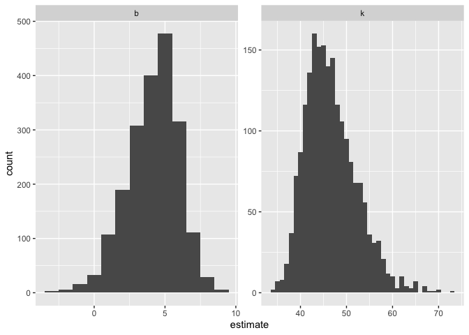
Interestingly, we get a left-skewed distribution for b and a right-skewed distribution for k.
Now, we can try plotting our models to see what the bootstrapped variance is, which gives us an idea as to what the true confidence interval should look like.
boot_aug <- boot_summary %>%
  mutate(augmented = map(model,augment)) %>%
  unnest(augmented)

ggplot(boot_aug, aes(wt,mpg)) +
  geom_line(aes(y = .fitted, group = id), alpha = .2, col = "red") +
  geom_point()
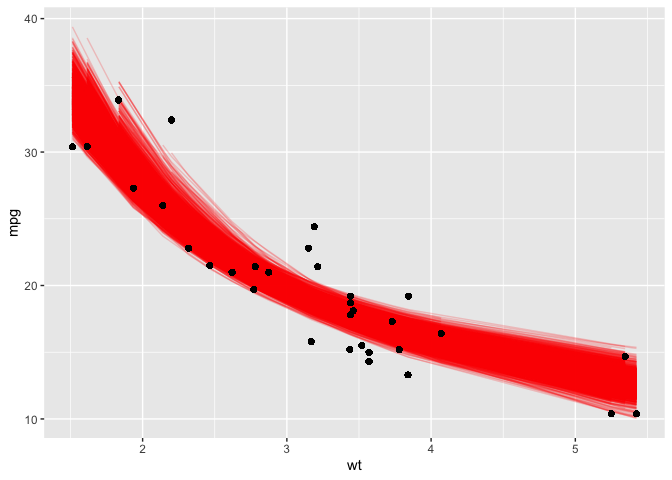
And look at that! We are given a great idea as to what the most likely range of regression curves would realistically be had we more data.