Time Series Analysis: Cardiovascular Mortality from the LA Pollution study

Background

This data comes from the astsa package in R, developed by Dr. David Stoffer who is one of the foremost Statisticians specializing in Time Series Analysis.

Description

Average weekly cardiovascular mortality in Los Angeles County; 508 six-day smoothed averages obtained by filtering daily values over the 10 year period 1970-1979.

library(astsa)
data("cmort")
tsplot(cmort,
       main = "Cardiovascular Mortality in Los Angeles (1970-1979)",
       ylab = "Mortality",
       xlab = "Year")

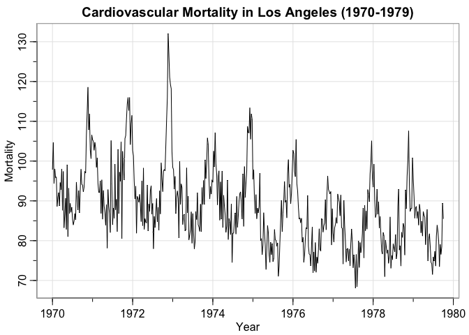
Note that there is a slight downward trend in the data as the city gets a better hold on pollution, indicating a non-constant mean. This breaks our assumption of stationarity. So, we difference the data to stabilize the mean.

tsplot(diff(cmort),
       main = "Differenced Cardiovascular Mortality in Los Angeles (1970-1979)",
       ylab = "Differenced Mortality",
       xlab = "Year")

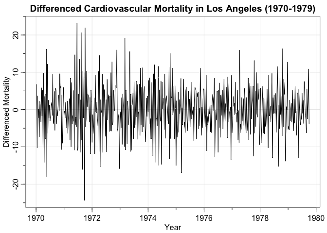
This is more like it! We have a stationary series and by observation we see the variance is stable, so no need for a logarithmic transformation.

P/ACF & Model Selection

In order to know the parameters of our ARIMA model, we need to examine its P/ACF graphs.

invisible(acf2(diff(cmort)))

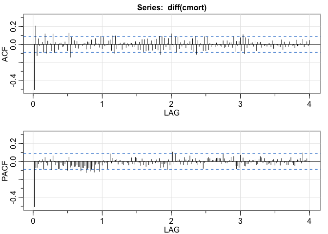
Note that the ACF trails off and the PACF cuts off at lag 1. We don’t see any seasonality. Additionally, the oscillatory nature of the ACF indicates that the model parameter will be negative.

This implies an ARIMA(1,1,0) model. We can use the sarima() function using these parameters.

sarima(cmort,1,1,0,no.constant = T)

## $fit
## 
## Call:
## stats::arima(x = xdata, order = c(p, d, q), seasonal = list(order = c(P, D, 
##     Q), period = S), include.mean = !no.constant, transform.pars = trans, fixed = fixed, 
##     optim.control = list(trace = trc, REPORT = 1, reltol = tol))
## 
## Coefficients:
##           ar1
##       -0.5064
## s.e.   0.0383
## 
## sigma^2 estimated as 33.81:  log likelihood = -1612.07,  aic = 3228.13
## 
## $degrees_of_freedom
## [1] 506
## 
## $ttable
##     Estimate     SE  t.value p.value
## ar1  -0.5064 0.0383 -13.2224       0
## 
## $AIC
## [1] 6.367124
## 
## $AICc
## [1] 6.36714
## 
## $BIC
## [1] 6.383805

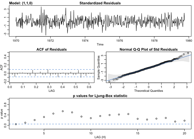
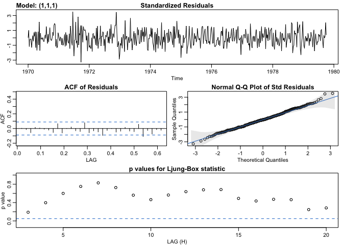
This model seems to fit well. The residuals are white noise and don’t have any significant autocorrelation left over. Further evidence of this can be seen from the high p-values in the series of Ljung-Box statistics. We also satisfy the normality condition as can be seen in the Q-Q plot.

The model parameter is estimated to be ϕ =  − 0.5064.

However, after reconsidering the ACF plot, one might argue that the PACF trails off instead of cutting off. In this case we would have an ARIMA(1,1,1) model. Let’s see how this compares to the current model.

sarima(cmort,1,1,1,no.constant = T)

## $fit
## 
## Call:
## stats::arima(x = xdata, order = c(p, d, q), seasonal = list(order = c(P, D, 
##     Q), period = S), include.mean = !no.constant, transform.pars = trans, fixed = fixed, 
##     optim.control = list(trace = trc, REPORT = 1, reltol = tol))
## 
## Coefficients:
##           ar1      ma1
##       -0.3779  -0.1717
## s.e.   0.0882   0.0967
## 
## sigma^2 estimated as 33.61:  log likelihood = -1610.58,  aic = 3227.15
## 
## $degrees_of_freedom
## [1] 505
## 
## $ttable
##     Estimate     SE t.value p.value
## ar1  -0.3779 0.0882 -4.2866  0.0000
## ma1  -0.1717 0.0967 -1.7749  0.0765
## 
## $AIC
## [1] 6.365197
## 
## $AICc
## [1] 6.365244
## 
## $BIC
## [1] 6.390218

They perform nearly identically well, and based on the Principle of Parsimony we should choose the simpler model, which is the ARIMA(1,1,0) model.

Forecasting

We can forecast this data now that we know the dynamics of the data.

invisible(sarima.for(cmort,n.ahead = 12,1,1,0))

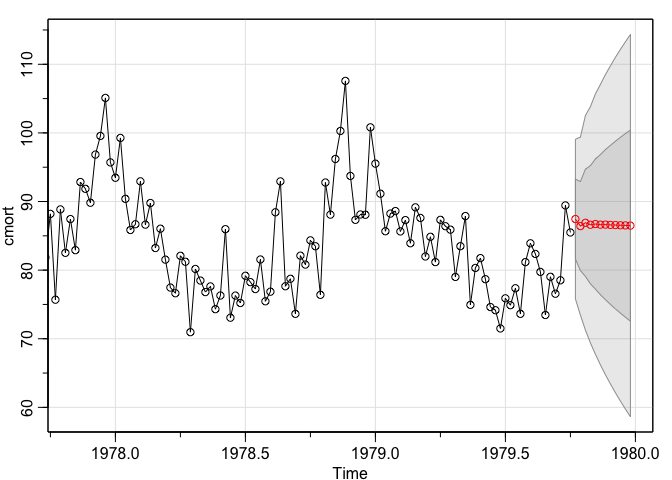
Notice how wide the bands are for the 90% and 95% C.I.’s. This is no surprise since the original data is highly variable.