Classifying Trees With Trees
Project Outset
This project uses the forest tree cover type data found on Kaggle. The directive is to classify each of the 7 possible forest cover types using this data. There are 500k+ records and 12 distinct fields (after reverting the One Hot Encoded fields back to a regular categorical).
This article will show how using sklearn can solve this problem. We will be focusing on the usage of trees and forests. Linear models and boosting techniques are not used, although they very well could be good solutions!
import pandas as pd
import numpy as np

from sklearn.datasets import fetch_covtype
from sklearn.model_selection import train_test_split
rs = 23
dat = fetch_covtype(as_frame=True)
data = dat.data.copy()
target = pd.Categorical(dat.target.copy())
As seen below, there is significant class imbalance. Classes 2 and 1 have over 85% of the records, leaving only 15% for the other 5 classes and even those are not uniformly distributed. What can we do? If we wanted to use linear models we would need to do quite a bit of pre-processing to be able to extract signal, and even that may not suffice. This can be costly when it comes to time and effort. Instead, we can try tree based models to find patterns. They are often preferred due to being more interpretable and not relying on assumptions like linearity.
dat.target.value_counts(normalize=True)
Cover_Type
2    0.487599
1    0.364605
3    0.061537
7    0.035300
6    0.029891
5    0.016339
4    0.004728
Name: proportion, dtype: float64
Before we jump into the modeling, there are some features that require some engineering.
Feature Engineering & EDA
First, we need to convert the Slope and Aspect fields to their trignometric sine and cosine values so that we can capture the true 2D orientation of the covers with respect to the direction they face as well as the angle to the sun. Otherwise, values that may seem different (such as 1 degree vs 360 degrees) will be misinterpreted by the model.
data["SinSlope"] = np.sin(np.radians(data["Slope"]))
data["SinAspect"] = np.sin(np.radians(data["Aspect"]))

data["CosSlope"] = np.cos(np.radians(data["Slope"]))
data["CosAspect"] = np.cos(np.radians(data["Aspect"]))

data.drop(columns = ['Aspect','Slope'],inplace=True)
Now we will convert the One Hot Encoded fields back to a pd.Categorical field. Since we will be using tree-based models we don’t need to introduce the additional dimensionality, nor do we need to center or scale numerical features. Plus it will make EDA easier
data_nohe = data.copy()

wild_cols = [col for col in data_nohe.columns if 'Wilderness_Area' in col]
data_nohe["Wilderness_Area"] = pd.Categorical(data_nohe[wild_cols].idxmax(axis=1).str.replace('Wilderness_Area_',''))#.astype(int)
soil_cols = [col for col in data_nohe.columns if 'Soil_Type' in col]
data_nohe["Soil_Type"] = pd.Categorical(data_nohe[soil_cols].idxmax(axis=1).str.replace('Soil_Type_',''))#.astype(pd.Categorical)

# need to drop the old one hot encoded fields using a for loop
data_nohe.drop(columns=wild_cols + soil_cols,inplace=True)

data_nohe.head()
| Elevation | Horizontal_Distance_To_Hydrology | Vertical_Distance_To_Hydrology | Horizontal_Distance_To_Roadways | Hillshade_9am | Hillshade_Noon | Hillshade_3pm | Horizontal_Distance_To_Fire_Points | SinSlope | SinAspect | CosSlope | CosAspect | Wilderness_Area | Soil_Type | |
|---|---|---|---|---|---|---|---|---|---|---|---|---|---|---|
| 0 | 2596.0 | 258.0 | 0.0 | 510.0 | 221.0 | 232.0 | 148.0 | 6279.0 | 0.052336 | 0.777146 | 0.998630 | 0.629320 | 0 | 28 |
| 1 | 2590.0 | 212.0 | -6.0 | 390.0 | 220.0 | 235.0 | 151.0 | 6225.0 | 0.034899 | 0.829038 | 0.999391 | 0.559193 | 0 | 28 |
| 2 | 2804.0 | 268.0 | 65.0 | 3180.0 | 234.0 | 238.0 | 135.0 | 6121.0 | 0.156434 | 0.656059 | 0.987688 | -0.754710 | 0 | 11 |
| 3 | 2785.0 | 242.0 | 118.0 | 3090.0 | 238.0 | 238.0 | 122.0 | 6211.0 | 0.309017 | 0.422618 | 0.951057 | -0.906308 | 0 | 29 |
| 4 | 2595.0 | 153.0 | -1.0 | 391.0 | 220.0 | 234.0 | 150.0 | 6172.0 | 0.034899 | 0.707107 | 0.999391 | 0.707107 | 0 | 28 |
Now we will look at how our features are correlated to see if we can drop any that seem redundant. Arbitrarily choose a threshold for what ‘redudant’ means to you. For this analysis I went with 75% correlation
# Calculate correlation matrix for important features
correlation_matrix = data_nohe.corr()

# Identify highly correlated pairs (e.g., above 0.9)
high_corr_pairs = [
    (feature1, feature2)
    for feature1 in correlation_matrix.columns
    for feature2 in correlation_matrix.index
    if feature1 != feature2 and abs(correlation_matrix.loc[feature1, feature2]) > 0.75
]
print("Highly Correlated Features:", high_corr_pairs)
Highly Correlated Features: [('Hillshade_9am', 'Hillshade_3pm'), ('Hillshade_9am', 'SinAspect'), ('Hillshade_3pm', 'Hillshade_9am'), ('Hillshade_3pm', 'SinAspect'), ('SinSlope', 'CosSlope'), ('SinAspect', 'Hillshade_9am'), ('SinAspect', 'Hillshade_3pm'), ('CosSlope', 'SinSlope')]
We see a number of combinations of features are quite correlated! They seem to be centered around Hillshade, a measurement of how much shade an area gets at a certain time of day, Aspect, which is the cardinal direction that the hill faces in degrees (converted to trig function), and Slope, which is the angle to the sun (also trig converted). This makes sense, since there is an obvious relationship between how much sun they’d receive and the direction they face and the angle they sit at! We can drop a few of these features that appear in combinations that are redundant:
Hillshare_9amHillshare_3pmSinSlope
data_nohe.drop(columns=['Hillshade_9am','Hillshade_3pm','SinSlope'],inplace=True)
data_nohe.head()
| Elevation | Horizontal_Distance_To_Hydrology | Vertical_Distance_To_Hydrology | Horizontal_Distance_To_Roadways | Hillshade_Noon | Horizontal_Distance_To_Fire_Points | SinAspect | CosSlope | CosAspect | Wilderness_Area | Soil_Type | |
|---|---|---|---|---|---|---|---|---|---|---|---|
| 0 | 2596.0 | 258.0 | 0.0 | 510.0 | 232.0 | 6279.0 | 0.777146 | 0.998630 | 0.629320 | 0 | 28 |
| 1 | 2590.0 | 212.0 | -6.0 | 390.0 | 235.0 | 6225.0 | 0.829038 | 0.999391 | 0.559193 | 0 | 28 |
| 2 | 2804.0 | 268.0 | 65.0 | 3180.0 | 238.0 | 6121.0 | 0.656059 | 0.987688 | -0.754710 | 0 | 11 |
| 3 | 2785.0 | 242.0 | 118.0 | 3090.0 | 238.0 | 6211.0 | 0.422618 | 0.951057 | -0.906308 | 0 | 29 |
| 4 | 2595.0 | 153.0 | -1.0 | 391.0 | 234.0 | 6172.0 | 0.707107 | 0.999391 | 0.707107 | 0 | 28 |
Let’s see which of the remaining features are correlated to the target. For our categorical features, Soil_Type and Wilderness_Area we will use Cramer’s V.
from dython.nominal import correlation_ratio
from scipy.stats import chi2_contingency

for i in data_nohe.columns:
    if i not in ['Soil_Type','Wilderness_Area']:
        cor_rat = correlation_ratio(data_nohe[i], target).round(2)
        print(i +" Correlation Ratio:", cor_rat)
    else:
        def cramers_v(contingency_table):
            chi2 = chi2_contingency(contingency_table)[0]
            n = contingency_table.sum().sum()
            phi2 = chi2/n
            min_dim = min(contingency_table.shape) - 1
            return np.sqrt(phi2 / min_dim)
        contingency_table = pd.crosstab(data_nohe[i], target)
        cramers_v = cramers_v(contingency_table).round(2)
        print(i + " Cramer's V:", cramers_v)
Elevation Correlation Ratio: 0.55
Horizontal_Distance_To_Hydrology Correlation Ratio: 0.09
Vertical_Distance_To_Hydrology Correlation Ratio: 0.1
Horizontal_Distance_To_Roadways Correlation Ratio: 0.19
Hillshade_Noon Correlation Ratio: 0.12
Horizontal_Distance_To_Fire_Points Correlation Ratio: 0.16
SinAspect Correlation Ratio: 0.06
CosSlope Correlation Ratio: 0.15
CosAspect Correlation Ratio: 0.06
Wilderness_Area Cramer's V: 0.44
Soil_Type Cramer's V: 0.47
Looks like Elevation has a relatively strong correlation ratio (.55) compared to the other variables. Next closest are Horizontal_Distance_To_Roadways (.19) and Horizontal_Distance_To_Fire_Points (.16). I expect these to stand out in the model when we look at the feature importance. The ones with lower ratios are likely to contibute very little and may be dropped to train the model again.
The two categorical variables, Wilderness_Area and Soil_Type, are calculated using Cramer’s V, which is different than a correlation ratio so the scales shouldn’t be compared. Looks like there not much of a relationship there, slightly worse than 50/50 where 0 is no relationship and 1 is perfect relationship.
Tree Based Models
Now we can split our training and testing data. We will use a 20% test size.
X_train, X_test, y_train, y_test = train_test_split(data_nohe,target,stratify=target,test_size=.2,random_state=rs)
We can begin the process of training and iterating on some models. We will start with a baseline model, a Decision Tree Classifier.
from sklearn.model_selection import RandomizedSearchCV, StratifiedKFold, cross_val_score
from sklearn.metrics import precision_recall_curve, confusion_matrix, classification_report
from sklearn.tree import DecisionTreeClassifier
from sklearn.model_selection import learning_curve
import matplotlib.pyplot as plt
strat_kfold = StratifiedKFold(n_splits=5, shuffle=True, random_state=rs)
To get the best model we will tune the model hyperparameters using RandomizedSearchCV with a StratifiedKFold object containing 10 splits and we will shuffle the data ahead of each iteration. This will ensure that each fold we train has class balance representative of our training data. We will randomly select 30 combinations of specified hyperparameters and the best model will be selected as defined by the f1_macro scoring metric. We choose this metric because we want to treat the performance on each class equally instead of weighting larger classes heavier. We choose f1 because we’d like to observe both recall and precision being high scoring and overall accuracy could be misleading due to the nature of imbalanced classes.
param_dist = {
    'max_depth': [20,40,80],
    'min_samples_leaf': [5,10,20,50],
    'min_samples_split': [10,30,50,100],
    'max_leaf_nodes': [5000,7000,10000],
    'criterion': ['entropy','gini']
}

rand_search = RandomizedSearchCV(
    estimator=DecisionTreeClassifier(),
    param_distributions=param_dist,
    n_iter=100,
    scoring='f1_macro',
    cv=strat_kfold,
    verbose=1,
    n_jobs=-1
)

rand_search.fit(X_train,y_train)

print(f"Best Parameters: {rand_search.best_params_}")
print(f"Best Cross-Validation f1: {rand_search.best_score_}")
f1 = rand_search.score(X_test, y_test)
print(f"Validation f1: {f1:.4f}")
Fitting 5 folds for each of 100 candidates, totalling 500 fits
Best Parameters: {'min_samples_split': 10, 'min_samples_leaf': 5, 'max_leaf_nodes': 10000, 'max_depth': 40, 'criterion': 'entropy'}
Best Cross-Validation f1: 0.8833766879741359
Validation f1: 0.8917
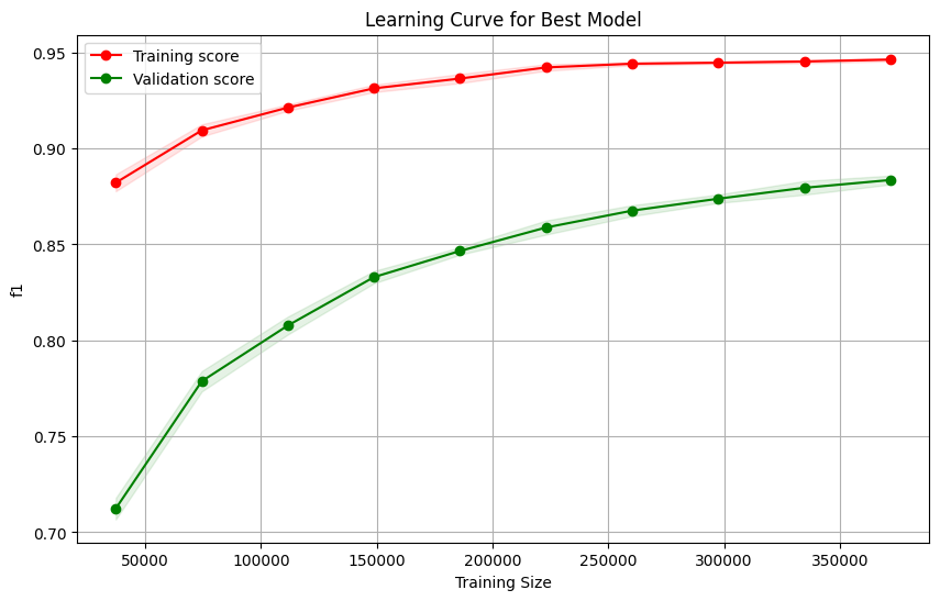
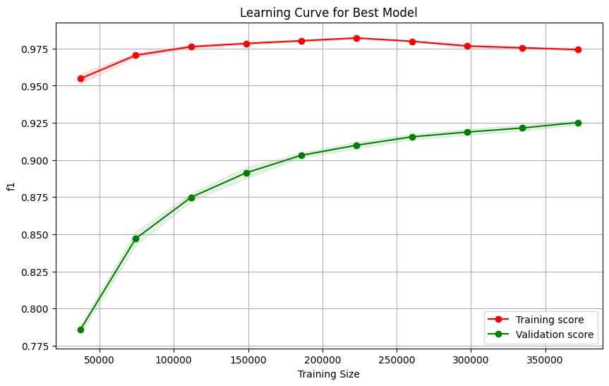
Let’s fit a learning curve using the best estimator to ensure we have a relatively stable model. This will show us whether we are overfitting or not, which trees tend to do.
train_sizes, train_scores, test_scores = learning_curve(rand_search.best_estimator_, X_train, y_train, cv=strat_kfold, scoring='f1_macro',train_sizes=np.linspace(0.1, 1.0, 10),  # Use 10 different training sizes
    n_jobs=-1)

# Compute mean and standard deviation for train/test scores
train_scores_mean = np.mean(train_scores, axis=1)
train_scores_std = np.std(train_scores, axis=1)
test_scores_mean = np.mean(test_scores, axis=1)
test_scores_std = np.std(test_scores, axis=1)

# print(f"Train Mean: {train_scores_mean}")
# print(f"Test Mean: {test_scores_mean}")
print(f"Diff: {(train_scores_mean[9] - test_scores_mean[9]).round(2)} ")

# Plot the learning curves
plt.figure(figsize=(10, 6))
plt.fill_between(train_sizes, train_scores_mean - train_scores_std,
                 train_scores_mean + train_scores_std, alpha=0.1, color="r")
plt.fill_between(train_sizes, test_scores_mean - test_scores_std,
                 test_scores_mean + test_scores_std, alpha=0.1, color="g")
plt.plot(train_sizes, train_scores_mean, 'o-', color="r", label="Training score")
plt.plot(train_sizes, test_scores_mean, 'o-', color="g", label="Validation score")

plt.title("Learning Curve for Best Model")
plt.xlabel("Training Size")
plt.ylabel("f1")
plt.legend(loc="best")
plt.grid()
plt.show()
Diff: 0.06
y_test_pred = rand_search.predict(X_test)#[X_train.columns]
print(classification_report(y_test,y_test_pred))
              precision    recall  f1-score   support

           1       0.93      0.93      0.93     42368
           2       0.94      0.94      0.94     56661
           3       0.92      0.93      0.93      7151
           4       0.86      0.81      0.83       549
           5       0.81      0.78      0.80      1899
           6       0.88      0.86      0.87      3473
           7       0.95      0.94      0.94      4102

    accuracy                           0.93    116203
   macro avg       0.90      0.88      0.89    116203
weighted avg       0.93      0.93      0.93    116203
After using the model to predict on our held out dataset, X_test, we can see that the model did not overfit (too much) and performed similarly to the validation sets from our folds observed in the learning curve. The smaller classes tend to struggle in performance, which is explained by the fact that this model being too simple to notice smaller nuanced patterns.
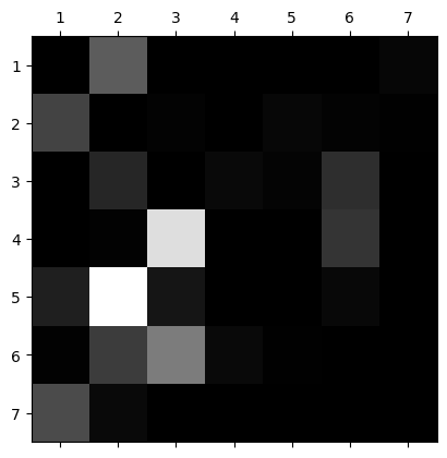
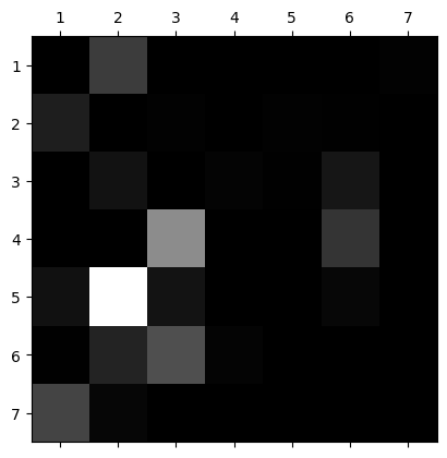
We can visualize the confusion matrix to get a better sense for how the model is mis-identifying them. We can see that class 5 is being identified as class 2 pretty frequently. Similar story for classes 4 and 6 being predicted as class 3.
conf_mx = confusion_matrix(y_test,y_test_pred)
row_sums = conf_mx.sum(axis=1,keepdims=True)
norm_conf_mx = conf_mx/row_sums
np.fill_diagonal(norm_conf_mx,0)
norm_conf_mx.round(3)
plt.matshow(norm_conf_mx,cmap=plt.cm.gray)
_ = plt.xticks(ticks=np.arange(7),labels=np.linspace(1,7,7).astype(int))
_ = plt.yticks(ticks=np.arange(7),labels=np.linspace(1,7,7).astype(int))
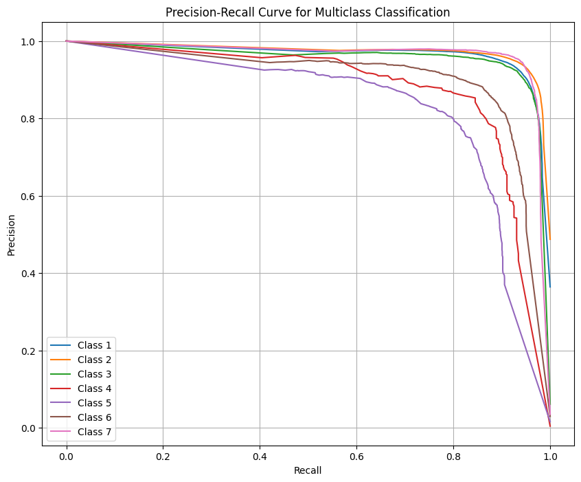
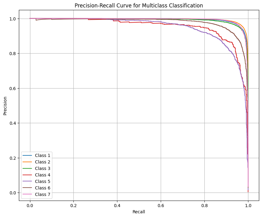
Let’s look at the Precision Recall curves to see how we are trading off the two as the proability threshold shifts. We see that the larger classes don’t trade off much if any Recall for Precision. However, the smaller classes perform poorly (relatively speaking) for both Precision and Recall.
# Initialize a plot
y_test_score = rand_search.predict_proba(X_test)
plt.figure(figsize=(10, 8))

# Calculate and plot the Precision-Recall curve for each class
classes = np.unique(dat.target)
for i, class_label in enumerate(classes):
    # Binary target: 1 if the current class, 0 otherwise
    y_test_binary = (y_test == class_label).astype(int)

    # Precision and recall for the current class
    precision, recall, _ = precision_recall_curve(y_test_binary, y_test_score[:, i])

    # Plot
    plt.plot(recall, precision, label=f'Class {class_label}')

# Customize the plot
plt.xlabel('Recall')
plt.ylabel('Precision')
plt.title('Precision-Recall Curve for Multiclass Classification')
plt.legend(loc="best")
plt.grid(True)
plt.show()
Below we see that there are a few features not offering a ton of information to the model. We can arbitraily set that threshold to determine what to get rid of from the model. That threshold will be 3.5%. Let’s see if we can either improve performance (ie f1 macro increases) or the model generalizes. We’ll use the same model parameters.
feature_importances = rand_search.best_estimator_.feature_importances_

feature_names = X_train.columns
importances_df = pd.DataFrame({
    'Feature': feature_names,
    'Importance': feature_importances.round(3)
}).sort_values(by='Importance', ascending=False)

importances_df
| Feature | Importance | |
|---|---|---|
| 0 | Elevation | 0.415 |
| 5 | Horizontal_Distance_To_Fire_Points | 0.128 |
| 3 | Horizontal_Distance_To_Roadways | 0.127 |
| 10 | Soil_Type | 0.119 |
| 1 | Horizontal_Distance_To_Hydrology | 0.049 |
| 2 | Vertical_Distance_To_Hydrology | 0.037 |
| 9 | Wilderness_Area | 0.036 |
| 8 | CosAspect | 0.031 |
| 6 | SinAspect | 0.025 |
| 4 | Hillshade_Noon | 0.017 |
| 7 | CosSlope | 0.016 |
# {'min_samples_split': 10, 'min_samples_leaf': 5, 'max_leaf_nodes': 10000, 'max_depth': 80, 'criterion': 'entropy'}
X_new = X_train[importances_df[importances_df["Importance"] > .035]['Feature']]
clf = DecisionTreeClassifier(max_depth=80, min_samples_leaf=5, min_samples_split=10, max_leaf_nodes=10000, criterion='entropy')
cross_val_score(clf,X_new,y_train,cv=strat_kfold,n_jobs=-1,verbose=2,scoring='f1_macro').mean().round(2)
[Parallel(n_jobs=-1)]: Using backend LokyBackend with 8 concurrent workers.


[CV] END .................................................... total time=   4.7s
[CV] END .................................................... total time=   4.7s
[CV] END .................................................... total time=   4.7s
[CV] END .................................................... total time=   4.7s
[CV] END .................................................... total time=   4.8s


[Parallel(n_jobs=-1)]: Done   2 out of   5 | elapsed:    4.9s remaining:    7.4s
[Parallel(n_jobs=-1)]: Done   5 out of   5 | elapsed:    4.9s finished


np.float64(0.88)
train_sizes, train_scores, test_scores = learning_curve(clf, X_new, y_train, cv=strat_kfold, scoring='f1_macro',train_sizes=np.linspace(0.1, 1.0, 10),  # Use 10 different training sizes
    n_jobs=-1)

# Compute mean and standard deviation for train/test scores
train_scores_mean = np.mean(train_scores, axis=1)
train_scores_std = np.std(train_scores, axis=1)
test_scores_mean = np.mean(test_scores, axis=1)
test_scores_std = np.std(test_scores, axis=1)

# print(f"Train Mean: {train_scores_mean}")
# print(f"Test Mean: {test_scores_mean}")
print(f"Diff: {(train_scores_mean[9] - test_scores_mean[9]).round(2)} ")

# Plot the learning curves
plt.figure(figsize=(10, 6))
plt.fill_between(train_sizes, train_scores_mean - train_scores_std,
                 train_scores_mean + train_scores_std, alpha=0.1, color="r")
plt.fill_between(train_sizes, test_scores_mean - test_scores_std,
                 test_scores_mean + test_scores_std, alpha=0.1, color="g")
plt.plot(train_sizes, train_scores_mean, 'o-', color="r", label="Training score")
plt.plot(train_sizes, test_scores_mean, 'o-', color="g", label="Validation score")

plt.title("Learning Curve for Best Model")
plt.xlabel("Training Size")
plt.ylabel("f1")
plt.legend(loc="best")
plt.grid()
plt.show()
Diff: 0.06
clf.fit(X_new,y_train)
y_test_pred = clf.predict(X_test[X_new.columns])
print(classification_report(y_test,y_test_pred))
              precision    recall  f1-score   support

           1       0.93      0.93      0.93     42368
           2       0.94      0.94      0.94     56661
           3       0.91      0.93      0.92      7151
           4       0.86      0.81      0.83       549
           5       0.82      0.79      0.80      1899
           6       0.87      0.84      0.85      3473
           7       0.94      0.93      0.94      4102

    accuracy                           0.93    116203
   macro avg       0.90      0.88      0.89    116203
weighted avg       0.93      0.93      0.93    116203
X_new.columns
Index(['Elevation', 'Horizontal_Distance_To_Fire_Points',
       'Horizontal_Distance_To_Roadways', 'Soil_Type',
       'Horizontal_Distance_To_Hydrology', 'Vertical_Distance_To_Hydrology',
       'Wilderness_Area'],
      dtype='object')
It looks like anything from that model that was contributing less than 3.5% really was not helping the model much. Getting rid of them allows us to maintain the same performance. Additionally it seems like our model is not unnecessarily overfitting either. We could likely reduce the gap to about 5% on the last run in the learning curve but the trade off in f1 macro wouldn’t be worth it. Seems like we have struck a good balance.
However, you can see that the validation curve has not plateaued quite yet. So this could mean that there is more juice to squeeze. We can try to get it by using more complex models like random forests or boosted trees. Let’s see.
Forests
A single tree can be very effective as seen above. But there may be room to improve results without needing to get into sampling techniques. Perhaps the problem with the 3 classes we observed lower performance for is due to lack of complexity in the model itself and not some issue with the input data. Let’s see.
from sklearn.ensemble import RandomForestClassifier
param_dist = {
    'max_depth': [50,75,100],
    'max_samples': [.6,.75,.9],
    'min_samples_leaf': [2,3,5],
    'min_samples_split': [5,10],
    'max_leaf_nodes': [5000,7500,10000],
    'max_features': ['sqrt','log2',.6,.8],
    'n_estimators': [20,50,100]
}

rand_search = RandomizedSearchCV(
    estimator=RandomForestClassifier(),
    param_distributions=param_dist,
    n_iter=25,
    scoring='f1_macro',
    cv=strat_kfold,
    verbose=1,
    random_state=rs,
    n_jobs=-1
)

rand_search.fit(X_train,y_train)
print(f"Best Parameters: {rand_search.best_params_}")
print(f"Best Cross-Validation f1: {rand_search.best_score_}")
f1 = rand_search.score(X_test, y_test)
print(f"Validation f1: {f1:.4f}")
Fitting 5 folds for each of 25 candidates, totalling 125 fits
Best Parameters: {'n_estimators': 50, 'min_samples_split': 5, 'min_samples_leaf': 2, 'max_samples': 0.75, 'max_leaf_nodes': 10000, 'max_features': 0.8, 'max_depth': 100}
Best Cross-Validation f1: 0.9242684279452815
Validation f1: 0.9267
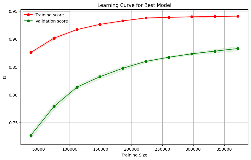
train_sizes, train_scores, test_scores = learning_curve(rand_search.best_estimator_, X_train, y_train, cv=strat_kfold, scoring='f1_macro',train_sizes=np.linspace(0.1, 1.0, 10),  # Use 10 different training sizes
    n_jobs=-1) #.best_estimator_

# Compute mean and standard deviation for train/test scores
train_scores_mean = np.mean(train_scores, axis=1)
train_scores_std = np.std(train_scores, axis=1)
test_scores_mean = np.mean(test_scores, axis=1)
test_scores_std = np.std(test_scores, axis=1)

print(f"Diff: {(train_scores_mean[9] - test_scores_mean[9]).round(2)} ")

# Plot the learning curves
plt.figure(figsize=(10, 6))
plt.fill_between(train_sizes, train_scores_mean - train_scores_std,
                 train_scores_mean + train_scores_std, alpha=0.1, color="r")
plt.fill_between(train_sizes, test_scores_mean - test_scores_std,
                 test_scores_mean + test_scores_std, alpha=0.1, color="g")
plt.plot(train_sizes, train_scores_mean, 'o-', color="r", label="Training score")
plt.plot(train_sizes, test_scores_mean, 'o-', color="g", label="Validation score")

plt.title("Learning Curve for Best Model")
plt.xlabel("Training Size")
plt.ylabel("f1")
plt.legend(loc="best")
plt.grid()
plt.show()
Diff: 0.05
# y_test_pred = cross_val_predict(rand_search.best_estimator_,X_test,y_test,cv=strat_kfold)
y_test_pred = rand_search.best_estimator_.predict(X_test)
conf_mx = confusion_matrix(y_test,y_test_pred)
print(classification_report(y_test,y_test_pred))
              precision    recall  f1-score   support

           1       0.96      0.95      0.96     42368
           2       0.96      0.97      0.96     56661
           3       0.95      0.96      0.95      7151
           4       0.92      0.85      0.89       549
           5       0.93      0.77      0.84      1899
           6       0.94      0.91      0.92      3473
           7       0.97      0.94      0.96      4102

    accuracy                           0.96    116203
   macro avg       0.95      0.91      0.93    116203
weighted avg       0.96      0.96      0.96    116203
Alright so we do see a pretty good boost in performance using the random forest. This model takes significantly longer to train but it is worth the tradeoff since the precision is significantly better and we get improvements in recall along with it. Interestingly, though, the recall for class 5 did not improve. It actually went down by 1%. This class must have some significant overlaps in features with class 2.
In the below confusion matrix you can see that 374 of the 1899 records from class 5 are going to class 2. We could address this by adding some complexity to the random forest such as allowing all of the features to be trained instead of limiting it to 3/4 (at most) or by adding some iterations to the cv search. This is costly, though, and may not be worth it.
conf_mx
array([[40337,  1922,     1,     0,    15,     3,    90],
       [ 1300, 55092,   106,     4,    87,    56,    16],
       [    0,    97,  6899,    24,    10,   121,     0],
       [    0,     0,    58,   469,     0,    22,     0],
       [   25,   366,    28,     0,  1469,    11,     0],
       [    4,    93,   207,    13,     1,  3155,     0],
       [  213,    19,     0,     0,     0,     0,  3870]])
row_sums = conf_mx.sum(axis=1,keepdims=True)
norm_conf_mx = conf_mx/row_sums
np.fill_diagonal(norm_conf_mx,0)
norm_conf_mx.round(3)
plt.matshow(norm_conf_mx,cmap=plt.cm.gray)
_ = plt.xticks(ticks=np.arange(7),labels=np.linspace(1,7,7).astype(int))
_ = plt.yticks(ticks=np.arange(7),labels=np.linspace(1,7,7).astype(int))
We confirm the improvement in performance by seeing how the PR curves have shifted further to the top right corner indicating the model is able to further minimize the trade off particularly for those smaller classes.
y_test_score = rand_search.predict_proba(X_test)
# Initialize a plot
plt.figure(figsize=(10, 8))

# Calculate and plot the Precision-Recall curve for each class
classes = np.unique(dat.target)
for i, class_label in enumerate(classes):
    # Binary target: 1 if the current class, 0 otherwise
    y_test_binary = (y_test == class_label).astype(int)

    # Precision and recall for the current class
    precision, recall, _ = precision_recall_curve(y_test_binary, y_test_score[:, i])

    # Plot
    plt.plot(recall, precision, label=f'Class {class_label}')

# Customize the plot
plt.xlabel('Recall')
plt.ylabel('Precision')
plt.title('Precision-Recall Curve for Multiclass Classification')
plt.legend(loc="best")
plt.grid(True)
plt.show()
If we wanted to go further we could try some boosting techniques like AdaBoost or lightgbm or xgboost. This could be a good choice due to their nature which is that they focus on the poor performing classes, like class 5 in this case. The tradeoff, of course, is the risk for more overfitting and it being very computationally expensive.